CFD-FVM-09: Solution algorithms for pressure-velocity coupling in steady flows

Introduction

Considering the equations governing a two-dimensional laminar steady flow:

• The convective terms of the momentum equations contain non-linear quantities
• All three equations are intricately coupled because every velocity component appears in each momentum equation and in the continuity equation.

In this case coupling between pressure and velocity introduces a constraint in the solution of the flow field: if the correct pressure field is applied in the momentum equations the resulting velocity field should satisfy continuity.

The staggered grid

If velocities and pressures are both defined at the nodes of an ordinary control volume a highly non-uniform pressure field can act like a uniform field in the discretised momentum equations.

The idea of a staggered grid is to evaluate scalar variables, such as pressure, density, temperature etc., at ordinary nodal points but to calculate velocity components on staggered grids centred around the cell faces

Scalar nodes locate at the intersection of the grid lines, denoted by and . The velocity nodes are located at the intersection of a line defining a cell boundary and a grid line, denoted by and . For example,, the -face of the cell around point is defined by

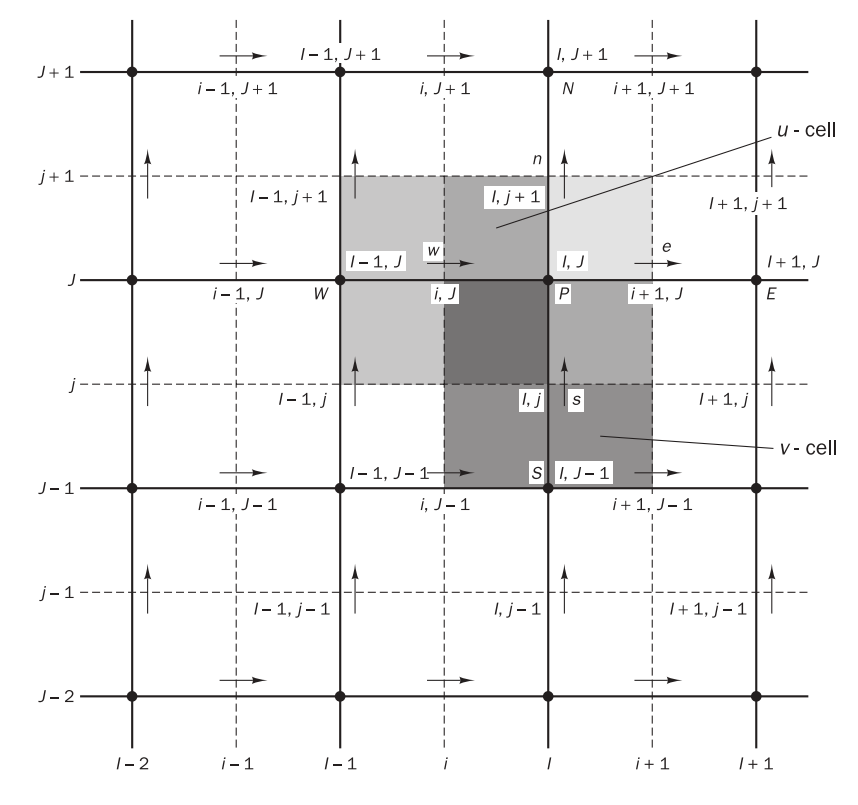
In the staggered grid arrangement, the pressure nodes coincide with the cell faces of the velocity-control volume, thus

A further advantage of the staggered grid arrangement is that it generates velocities at exactly the locations where they are required for the scalar transport–convection–diffusion computations. Hence, no interpolation is needed to calculate velocities at the scalar cell faces.

The momentum equations

We may use forward or backward staggered velocity grids. The uniform grids in above figure are backward staggered since the -location for the -velocity is at a distance of from the scalar node .

Expressed in the new co-ordinate system the discretised -momentum equation for the velocity at location is given by

or

In the new numbering system the , , and neighbours involved in the summation are , , and respectively. Their locations and the prevailing velocities are shown in more detail in below figure.

The values of coefficients and may be calculated with any of the differencing methods (upwind, hybrid, QUICK, TVD) suitable for convection–diffusion problems. The coefficients contain combinations of the convective flux per unit mass and the diffusive conductance at -control volume cell faces.

The formulae show that where scalar variables or velocity components are not available at a -control volume cell face, a suitable two- or four-point average is formed over the nearest points where values are available

By analogy the -momentum equation becomes

Again at each iteration level the values of are computed using the - and - velocity components resulting from the previous iteration.

The SIMPLE algorithm

The acronym SIMPLE stands for Semi-Implicit Method for PressureLinked Equations. To initiate the SIMPLE calculation process a pressure field is guessed. Discretised momentum equations are solved using the guessed pressure field to yield velocity components and as follows:

Now we define the correction as the difference between correct pressure field and the guessed pressure field , so that

Similarly,

By subtracting, we have

Hence,

Omission of and is the main approximation of the SIMPLE algorithm. We obtain


where

To update the velocities, we have

Continuity is satisfied in discretised form for the scalar control volume as:

Subsitiuting the corrected velocities and rearranging the terms, we have

where and the coefficient are given by

Above equation represents the discretised continuity equation as an equation for pressure correction .

The omission of terms such as in the derivation does not affect the final solution because the pressure correction and velocity corrections will all be zero in a converged solution, giving and and . The pressure correction equation is susceptible to divergence unless some
under-relaxation is used during the iterative process, and new, improved, pressures are obtained with

where is the under-relaxation factor. The velocities are also under-relaxed. The iteratively improved velocity components and are obtained from


where and are the velocities from the previous iteration.

The SIMPLE algorithm is an iterative procedure for the calculation of pressure and velocity fields. Starting from an initial pressure field its principal steps are:

• solve discretised momentum equation to yield intermediate velocity field
• solve discretised continuity equation in the form of an equation for pressure correction
• correct pressure and velocity by means of
  
  
  
• solve all other discretised transport equations for scalars
• repeat until , , and fields have all converged.

The SIMPLER algorithm

The SIMPLE Revised (SIMPLER) is an improved version of SIMPLE. In this algorithm the discretised continuity equation is used to derive a discretised equation for pressure, instead of a pressure correction equation as in SIMPLE. Thus the intermediate pressure field is obtained directly without the use of a correction

The SIMPLEC algorithm

The SIMPLEC (SIMPLE-Consistent) algorithm of Van Doormal and Raithby (1984) follows the same steps as the SIMPLE algorithm, with the difference that the momentum equations are manipulated so that the SIMPLEC velocity correction equations omit terms that are less significant than those in SIMPLE.

where

The PISO algorithm

The PISO algorithm, which stands for Pressure Implicit with Splitting of Operators, of Issa (1986) is a pressure–velocity calculation procedure developed originally for non-iterative computation of unsteady compressible flows. PISO involves one predictor step and two corrector steps and may be seen as an extension of SIMPLE, with a further corrector step to enhance it.

Predictor step

A guessed or intermediate pressure field , same as SIMPLE.

Corrector step 1

The first corrector step of SIMPLE is introduced to give a velocity field which satisfies the discretised continuity equation.

Corrector step 2

To enhance the SIMPLE procedure PISO performs a second corrector step. A twice-corrected velocity field may be obtained by solving the momentum equations once more:

Performing similar steps as SIMPLE, we have


where is the second pressure correction so that may be obtained by

The PISO algorithm solves the pressure correction equation twice so the method requires additional storage for calculating the source term of the second pressure correction equation. As before, under-relaxation is required with the above procedure to stabilise the calculation process. Although this method implies a considerable increase in computational effort it has been found to be efficient and fast.

General comments on SIMPLE, SIMPLER, SIMPLEC and PISO

• In SIMPLE, the pressure correction is satisfactory for correcting velocities but not so good for correcting pressure.
• Hence the improved procedure SIMPLER uses the pressure corrections to obtain velocity corrections only. A separate, more effective, pressure equation is solved to yield the correct pressure field.