CFD-FVM-08: Higher-order Differencing Schemes for Convection-diffusion Problems

Quadratic upwind differencing scheme: the QUICK scheme

For example, when , we have

When , we have

Combining this scheme for convective term and central differencing scheme for diffusive term, the discretization of the convection-diffusion equation for and can be

which can be rearranged to give

In a standard form, we can write

where

For and , we have

The QUICK scheme for one-dimensional convection–diffusion problems can be summarised as follows:

with central coefficients

and

where for and for , and for and for .

Assessment of the QUICK scheme

The scheme uses consistent quadratic profiles – the cell face values of fluxes are always calculated by quadratic interpolation between two bracketing nodes and an upstream node – and is therefore conservative.
The main coefficients ( and ) are not guaranteed to be positive and the coefficients and are negative.
Tri-diagonal matrix solution methods are not directly applicable.

Stability problems of the QUICK scheme and remedies

These formulations all involve placing troublesome negative coefficients in the source term so as to retain positive main coefficients.

The Hayase et al. (1992) QUICK scheme can be summarised as follows:

The discretisation equation takes the form

with central coefficients

and

where for and for , and for and for .

General comments on the QUICK differencing scheme

greater formal accuracy
retains the upwind-weighted characteristics
can lead to subtle problems: for example, they could give rise to negative turbulence kinetic energy () in model computations.

TVD schemes

Generalisation of upwind-biased discretisation schemes

We assume that the flow is in the positive -direction, so .
Upwind differencing (UD) is . Involving two upstream nodes (linear upwind differencing, LUD) yields

These schemes can be considered as

UD plus a correction term
the sum of the UD convective flux plus an additional flux contribution .

The QUICK can be rearranged in this way to give

The central differencing (CD) can be rearranged in this way to give

In a more general form

For LUD

For QUICK

Then with , the general form of the east face value within a discretisation scheme for convective flux may be written as

Total variation and TVD schemes

For a scheme to preserve monotonicity

it must not create local extrema
the value of an existing local minimum must be non-decreasing and that of a local maximum must be non-increasing
In simple terms, monotonicity-preserving schemes do not create new undershoots and overshoots in the solution or accentuate existing extremes.

Consider the discrete data set shown in above figure. The total variation for this set of data is defined as

For monotonicity to be satisfied, this total variation must not increase. Monotonicity-preserving schemes have the property that the total variation of the discrete solution should diminish with time. Hence the term total variation diminishing or TVD. For transient problems, .

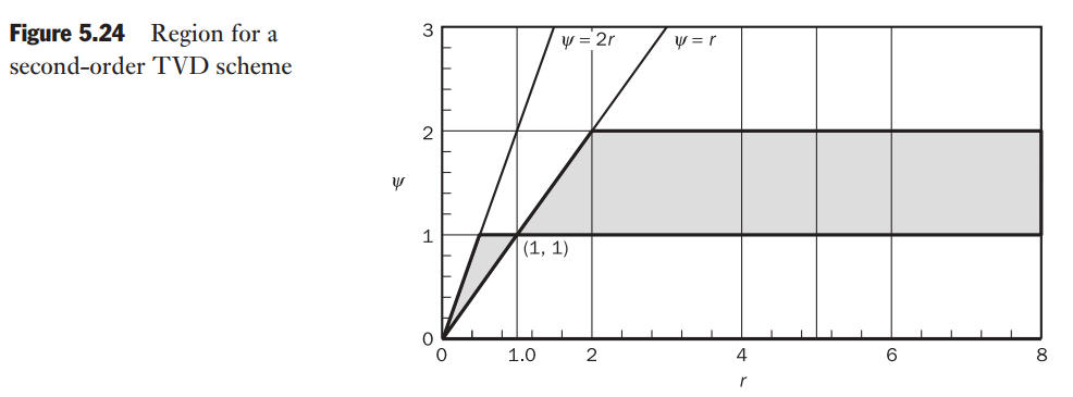
Criteria for TVD schemes

Sweby (1984) has given necessary and sufficient conditions for a scheme to be TVD in terms of the relationship:

If the upper limit is , so for TVD schemes .
If the upper limit is , so for TVD schemes .

the UD scheme is TVD
the LUD scheme is not TVD for
the CD scheme is not TVD for
the QUICK scheme is not TVD for and

The idea of designing a TVD scheme is to introduce a modification to the above schemes so as to force the relationship to remain within the shaded region for all possible values of . This would imply that, in order to make the scheme TVD, we must constrain or limit the range of possible values of the additional convective flux , which was originally introduced to make the scheme higher-order. Hence, the function is called a flux limiter function.

Sweby (1984): The flux limiter function of a second-order accurate scheme should pass through the point (1, 1) in the diagram.

Sweby finally introduced the symmetry property for limiter functions:

A limiter function that satisfies the symmetry property ensures that backward- and forward-facing gradients are treated in the same fashion without the need for special coding.

Flux limiter functions

Name	Limiter function	Source
Van Leer		Van Leer (1974)
Van Albada		Van Albada (1982)
Min-Mod		Roe (1985)
SUPERBEE		Roe (1985)
Sweby		Sweby (1984)
QUICK		Leonard (1988)
UMIST		Lien and Leschziner (1993)

It is relatively easy to verify that Leonard’s QUICK limiter function is the only one that is non-symmetric, whereas all the others are symmetric limiters

Implementation of TVD schemes

Consider the one-dimensional convection–diffusion equation again

The diffusion term is discretised using central differencing as before, we have

For , using TVD schemes it may be written as

where

Substitution aboves into the equation gives

Rearranging gives

This can be written as

where

, and are those of the UD scheme, providing the numerical stability.

In a general form, we note and for and and for , then

In a more general form, we can write the TVD neighbour coefficients as

and the TVD deferred correction source term as

where for and for ; for and for .

Treatment at the boundaries

Leonard mirror node extrapolation for the left (inlet/outlet) boundary gives

Extension to two and three dimensions

TVD scheme in a two-dimensional Cartesian grid:

with central coefficient

TVD neighbour coefficients:

and the TVD deferred correction source term:

where

The extension to three dimensions is straightforward.