CFD-FVM-07: The Finite Volume Method for Convection-diffusion Problems
Introduction
The steady convection–diffusion equation
Formal integration over a control volume gives
Steady one-dimensional convection and diffusion
We consider
satisfying the continuity equation
Consider the grid of
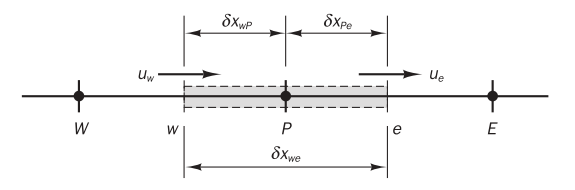
Then we have
It is convenient to define two variables
Using the central differencing we have
We also assume that the velocity field is ‘somehow known’.
The central differencing scheme
Let’s try the central scheme to compute the cell face values for the convective terms
Rearranging the terms we have
Further rearranging the terms we have
Writing to the form of
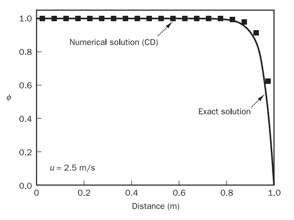
Example 1
A property

- case 1:
- case 2:
- case 3:
with 20 grid nodes.
Analytical solution:

For node 2, node 3 and node 4 we use the above conclusion. For node 1 we have
For node 5 we have
Note that
with
with
| Node | ||||
|---|---|---|---|---|
| 1 | 0 | |||
| 2, 3, 4 | 0 | 0 | ||
| 5 | 0 |
Case 1

Case 2

These oscillations are often called ‘wiggles’ in the literature
Case 3
It has reduced the
Properties of discretisation schemes
- Conservativeness
- Boundedness
- Transportiveness
Conservativeness
To ensure conservation of

Since
Boundedness
Scarborough (1958) has shown that a sufficient condition for a convergent iterative method can be expressed in terms of the values of the coefficients of the discretised equations:
If the differencing scheme produces coefficients that satisfy the above criterion the resulting matrix of coefficients is diagonally dominant.
- This states that in the absence of sources the internal nodal values of property
should be bounded by its boundary values. - Another essential requirement for boundedness is that all coefficients of the discretised equations should have the same sign (usually all positive).
Transportiveness
We define the non-dimensional cell Peclet number as a measure of the relative strengths of convection and diffusion:
- no convection and pure diffusion (
)

- no diffusion and pure convection (
) - in between

It is very important that the relationship between the directionality of influencing and the flow direction and magnitude of the Peclet number, known as the transportiveness, is borne out in the discretisation scheme.
Assessment of the central differencing scheme for convection-diffusion problems
Conservativeness: Satisfied
Boundedness: with
Transportiveness: The central differencing scheme introduces influencing at node P from the directions of all its neighbours to calculate the convective and diffusive flux. Thus the scheme does not recognise the direction of the flow or the strength of convection relative to diffusion. It does not possess the transportiveness property at high
The upwind differencing scheme
One of the major inadequacies of the central differencing scheme is its inability to identify flow direction.
The value of property
at a west cell face is always influenced by both and in central differencing.

Example 2
Solve the problem considered in Example 1 using the upwind differencing scheme for (i)
| Node | ||||
|---|---|---|---|---|
| 1 | 0 | |||
| 2, 3, 4 | 0 | 0 | ||
| 5 | 0 |
Case 1

Case 2

Assessment of the upwind differencing scheme
The upwind differencing scheme causes the distributions of the transported properties to become smeared. The resulting error has a diffusion-like appearance and is referred to as false diffusion.
Trials have shown that, in high Reynolds number, flows, false diffusion can be large enough to give physically incorrect results.
The hybrid differencing scheme
The central differencing scheme, which is second-order accurate, is employed for small Peclet numbers (
For example, for a west face,
The hybrid differencing formula for the net flux per unit area through the west face is as follows:
The general form of the discretised equation is
After some rearrangement it is easy to verify that the neighbour coefficients for the hybrid differencing scheme for steady one-dimensional convection–diffusion can be written as follows:
Hybrid differencing scheme for multi-dimensional convection-diffusion
The discretised equation that covers all cases is given by
with central coefficient
| One-dimensional | Two-dimensional | Three-dimensional | |
|---|---|---|---|
| 0 | |||
| 0 | |||
| 0 | 0 | ||
| 0 | 0 | ||
In the above expressions the values of
| Face | w | e | s | n | b | t |
|---|---|---|---|---|---|---|
The power-law scheme
In this scheme diffusion is set to zero when cell
For example, the net flux per unit area at the west control volume face is evaluated using
where
for
For