CFD-FVM-06: The Finite Volume Method for Diffusion Problems

Introduction

The governing equation of steady diffusion

The control volume integration

Finite volume method for one-dimensional steady state diffusion

The process is governed by

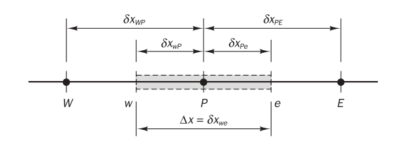
Step 1: Grid generation

The usual notations are shown as follows

Step 2: Discretisation

For the control volume defined above the integration is

Here is the cross-sectional area of the control volume face, is the volume and is the average value of source over the control volume.

For a uniform grid, the simplest way to get the value at the interface is the central differencing:

Then

The source term is approximated by a linear interpolation

Finally we have

Rearrange the equation

We assign

Then

Step 3: Solution of equations

Above discretised equations must be set up at each of the nodal points in order to solve a linear algebraic equations to obtain the solution.

Worked examples: onedimensional steady state diffusion

The equation governing one-dimensional steady state conductive heat transfer is

The source term can, for example, be heat generation due to an electrical current passing through the rod.

Example 1

No source term:

For node 2, 3 and 4, with

Integration of the equation over the control volume surrounding point 1 gives

Rearrange the equation yields with

The similar manner can be applied to point 5 with

All the coefficients and equations can form a matrix equation which can be solved by a linear algebraic solver. Then we can obtain the temperature distribution.

Example 2

A uniform heat generation of q:

Assuming that the dimensions in the - and -directions are so large that temperature gradients are significant in the -direction only.

For node 2, 3 and 4 we have

Rearrange the equation to the form of with

For node 1 we have

Rearrange the equation to the form of with

For node 5 we have

Rearrange the equation to the form of with

Example 3

We consider a cylindrical fin with uniform crosssectional area . The base is at a temperature of () and the end is insulated. The fin is exposed to an ambient temperature of . We have

where is the heat transfer coefficient and is the perimeter of the fin.

Since the governing equation can be written as

Integration of the above equation over a control volume gives

The second integral due to the source term in the equation is evaluated by assuming that the integrand is locally constant within each control volume:

For node 2, 3 and 4 we have

Rearrange the equation to the form of with

For node 1 we have

Rearrange the equation to the form of with

For node 5 we have

Rearrange the equation to the form of with

Finite volume method for two-dimensional diffusion problems

Consider a two-dimensional steady diffusion problem

When the above equation is formally integrated over the control volume we obtain

Given the grid as

we have

Using the central difference we have

This yields the form of with

Finite volume method for three-dimensional diffusion problems

Steady state diffusion in a three-dimensional situation is governed by

Given the grid as

we have

Discretizing the above equation using the central difference we have

This yields the form of with

Summary

• The discretised equations have a general form:
  
  where means the neighbouring nodes.
• In all cases the coefficients around point P satisfy the following relation:
  
  with the values in below table

1D			0	0	0	0
2D					0	0
3D

• Source terms can be included by identifying their linearised form and specifying values for and .
• Boundary conditions are incorporated by suppressing the link to the boundary side and introducing the boundary side flux – exact or linearly approximated – through additional source terms and . For a one-dimensional control volume of width with a boundary B:
  • link cutting: set coefficient
  • source contributions:
    • fixed value :
      
      
    • fixed flux :