CFD-FVM-02: Classification of Physical Behaviours

First we distinguish two principal categories of physical behaviour:

Equilibrium problems
Marching problems

Equilibrium problems

These and many other steady state problems are governed by elliptic equations. The prototype elliptic equation is Laplace’s equation, which describes irrotational flow of an incompressible fluid and steady state conductive heat transfer. In two dimensions we have

A very simple example of heat conduction:

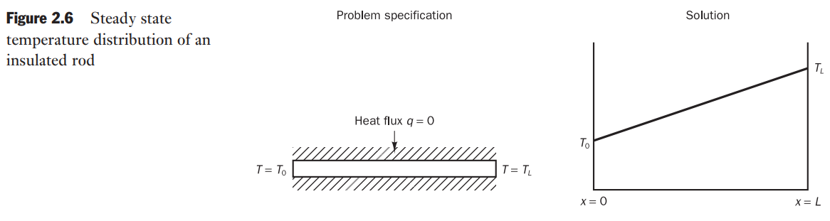
This problem is one-dimensional and governed by the equation .

Problems requiring data over the entire boundary are called boundary-value problems

Disturbance signals travel in all directions through the interior solution for elliptic equations. Consequently, the solutions to physical problems described by elliptic equations are always smooth even if the boundary conditions are discontinuous.

Marching problems

These problems are governed by parabolic or hyperbolic equations.

Parabolic equations

Parabolic equations describe time-dependent problems involving significant amounts of diffusion. The prototype parabolic equation is the diffusion equation

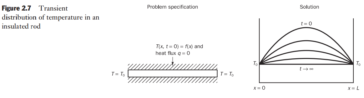
Initial conditions are needed in the entire rod and conditions on all its boundaries are required for all times . This type of problem is termed an initial–boundary-value problem.

The steady state is reached as time and is elliptic. This change of character can be easily seen by setting . The governing equation is now equal to the one governing the steady temperature distribution in the rod.

Hyperbolic equations

The prototype hyperbolic equation is the wave equation

It will be shown that disturbances at a point can only influence a limited region in space. The speed of disturbance propagation through an hyperbolic problem is finite and equal to the wave speed c. In contrast, parabolic and elliptic models assume infinite propagation speeds.

The role of characteristics in hyperbolic equations

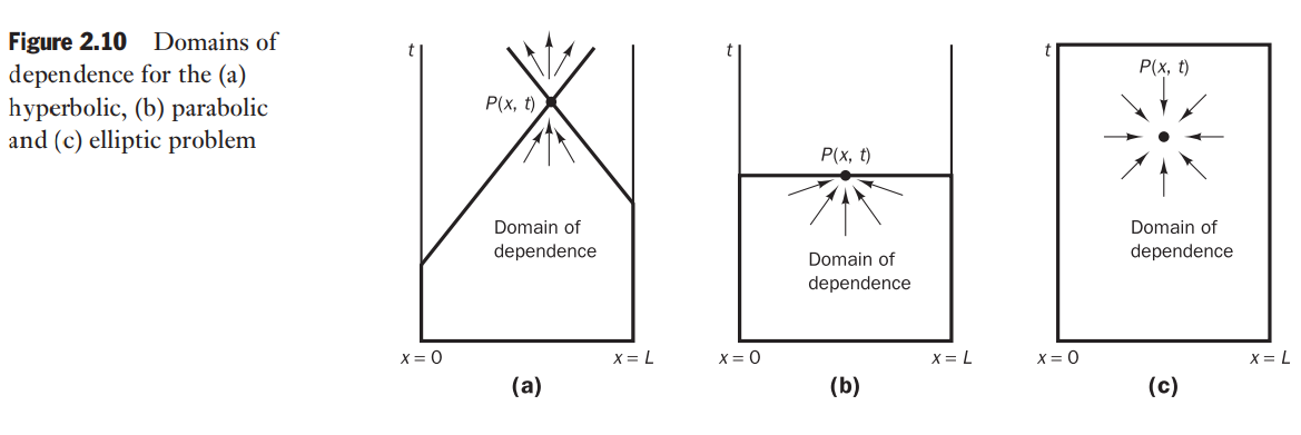
The way in which changes at one point affect events at other points depends on whether a physical problem represents a steady state or a transient phenomenon and whether the propagation speed of disturbances is finite or infinite.

Summary

Problem type	Equation type	Conditions	Solution domain	Sol. smoothness
Equilibrium problems	Eliptic	Boundary conditions	Closed domain	Always smooth
Marching problems with dissipation	Parabolic	Initial and boundary conditions	Open domain	Always smooth
Marching problem without dissipation	Hyperbolic	Initial and boundary conditions	Open domain	May be disconti- nuous

Classification method for simple PDEs

A practical method of classifying PDEs is developed for a general secondorder PDE in two co-ordinates and . Consider

The classification of a PDE is governed by the behaviour of its highestorder derivatives, so we need only consider the second-order derivatives.

By looking at the characteristic equation

Simple wave solutions occur if the characteristic equation below has two real roots:

	Equation type	Characteristics
	Hyperbolic	Two real characteristics
	Parabolic	One real characteristic
	Elliptic	No characteristics

when , or is dependent on , it also works. The type may be mixed (depends on )

independent variables

Given

Fletcher (1991) explains that the equation can be classified on the basis of the eigenvalues of a matrix with entries

if any eigenvalue : the equation is parabolic
if all eigenvalues and they are all of the same sign: the equation is elliptic
if all eigenvalues and all but one are of the same sign: the equation is hyperbolic

Classification of fluid flow equations

	Steady flow	Unsteady flow
Viscous flow	Elliptic	Parabolic
Inviscid flow	, elliptic , hyperbolic	Hyperbolic
Thin shear layers	Parabolic	Parabolic

For practical problems, the type might be mixed. Such flows may contain shockwave discontinuities and regions of subsonic (elliptic) flow and supersonic (hyperbolic) flow, whose exact locations are not
known a priori.

Auxiliary conditions for viscous fluid flow equations

Boundary conditions for compressible viscous flow

Initial conditions for unsteady flows:
- Everywhere in the solution region , and must be given at time .
Boundary conditions for unsteady and steady flows:
- On sold walls:
  - (no-slip condition)
  - (fixed temperature) or (fixed heat flux)
- On fluid boundaries:
  - inlet: , and must known as a function of position
  - outlet: and (stress continuity)

In the table subscripts and indicate directions normal (outward) and tangential to the boundary respectively and are the given surface stresses.

Outflow condition

specified pressure

Symmetry boundary condition:
Cyclic boundary condition: