CFD-FVM-01: Navier-Stokes Equations

整理自
Versteeg H K, Malalasekera W. An introduction to computational fluid dynamics: the finite volume method[M]. Pearson education, 2007.

Introduction

CFD codes are structured around the numerical algorithms that can tackle fluid flow problems.

All codes contain three main elements:

1. a pre-processor
2. a solver
3. a post-processor.

Solver

The most popular solution procedures are by the TDMA (tri-diagonal matrix algorithm) line-by-line solver of the algebraic equations and the SIMPLE algorithm to ensure correct linkage between pressure and velocity. Commercial codes may also give the user a selection of further, more recent, techniques such as Gauss–Seidel point iterative techniques with multigrid accelerators and conjugate gradient methods.

Conservation laws of fluid motion and boundary conditions

The governing equations of fluid flow represent mathematical statements of the conservation laws of physics:

• The mass of a fluid is conserved
• The rate of change of momentum equals the sum of the forces on a fluid particle (Newton’s second law)
• The rate of change of energy is equal to the sum of the rate of heat addition to and the rate of work done on a fluid particle (first law of thermodynamics)

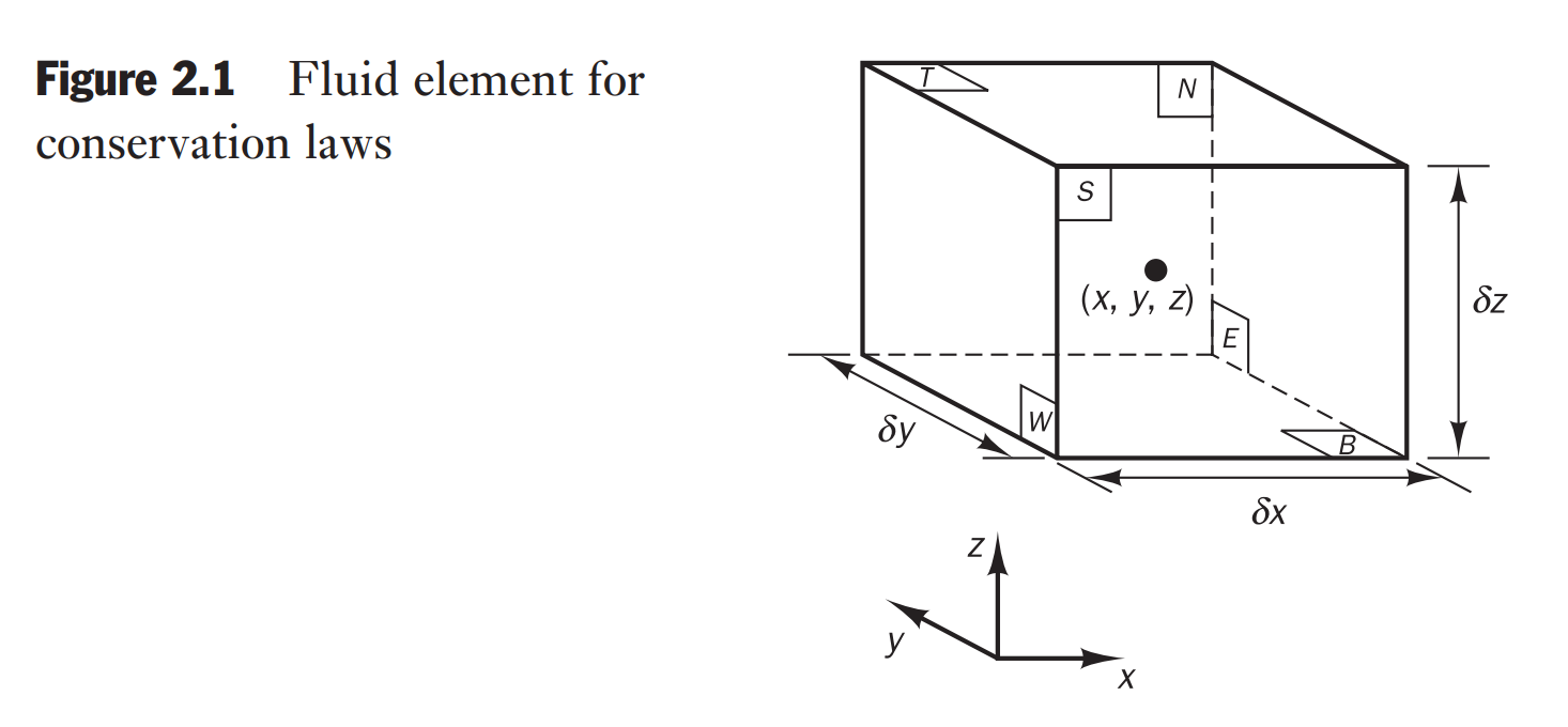
The element under consideration is so small that fluid properties at the faces can be expressed accurately enough by means of the first two terms of a Taylor series expansion. So, for example, the pressure at the and faces, which are both at a distance of from the element centre, can be expressed as

Mass conservation in three dimensions

Rate of increase of mass in fluid element = Net rate of flow of mass into fluid element

The Rate of increase of mass in the fluid element is

According to the figure

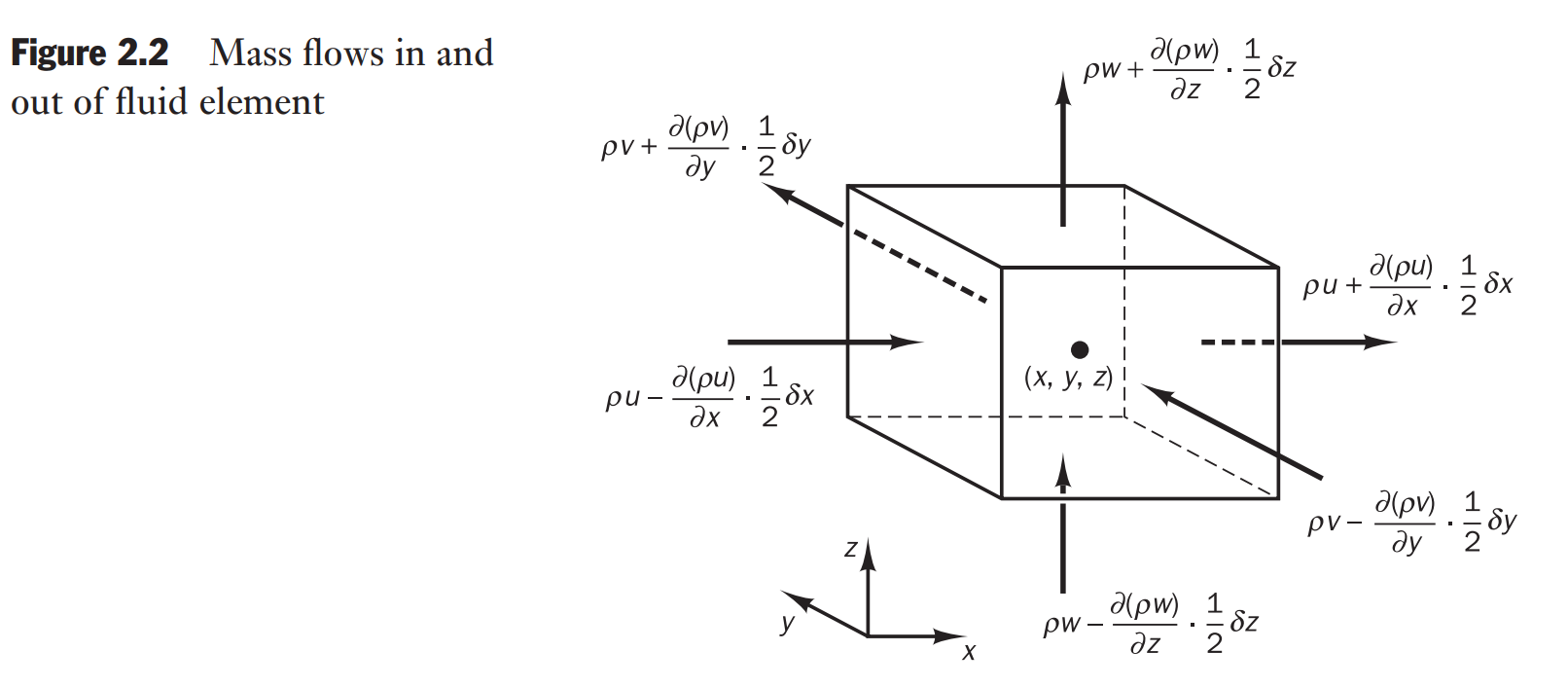
the Net rate of flow of mass into fluid element is

Divided by the element volume , yields

or in more compact vector notation

For an incompressible fluid (i.e. a liquid) the density is constant and the equation becomes

Rates of change following a fluid particle and for a fluid element

Let the value of a property per unit mass be denoted by , a function of the position of the particle and time . As in the case of the mass conservation equation, we are interested in developing equations for rates of change per unit volume. Ignore the derivation, we have

which is

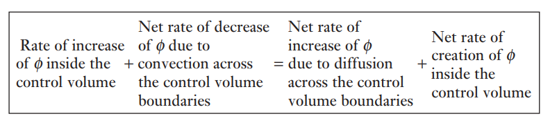
Rate of increase of of fluid element + Net rate of flow of of fluid element = Rate of increase of for a fluid particle

To construct the three components of the momentum equation and the energy equation the relevant entries for φ and their rates of change per unit volume are given below:

x-momentum
y-momentum
z-momentum
energy

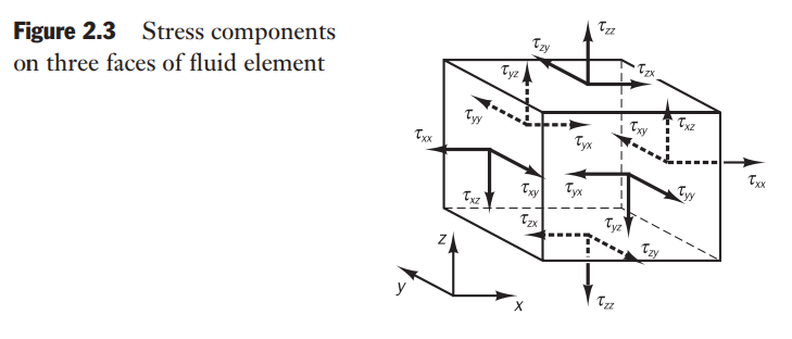
Momentum equation in three dimensions

Newton’s second law states that the rate of change of momentum of a fluid particle equals the sum of the forces on the particle:

Rate of increase of momentum of fluid particle = Sum of forces on fluid particle

• surface forces
  • pressure forces
  • viscous forces
  • gravity force (?)
• body forces
  • centrifugal force
  • Coriolis force
  • electromagnetic force

It is common practice to highlight the contributions due to the surface forces as separate terms in the momentum equation and to include the effects of body forces as source terms.

The suffices and in indicate that the stress component acts in the direction on a surface normal to the -direction.

On the pair of faces we have

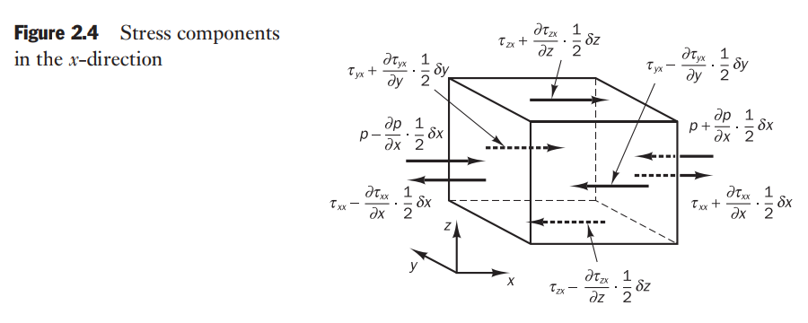
Of this sense, the net force in the -direction on the pair of faces is

Finally the net force in the x-direction on faces and is given by

The total force per unit volume on the fluid due to these surface stresses is equal to (divided by the volume )

Without considering the body forces in further detail their overall effect can be included by defining a source of -momentum per unit volume per unit time.

Hence,

usual sign convention takes a tensile stress to be the positive normal stress so that the pressure, which is by definition a compressive normal stress, has a minus sign.

Energy equation in three dimensions

Rate of increase of energy of fluid particle = Net rate of heat added to fluid particle + Net rate of work done on fluid particle

Work done by surface forces

The rate of work done on the fluid particle in the element by a surface force is equal to the product of the force and velocity component in the direction of the force. For -direction,

For - and -direction,

These yield the following total rate of work done on the fluid particle by
surface stresses:

Energy flux due to heat conduction

The heat flux vector has three components: , and . The unit of is .

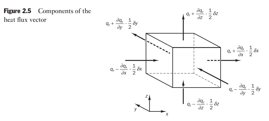
For face and (-direction):

For - and -direction:

The total rate of heat added to the fluid particle per unit volume due to heat flow across its boundaries (divided by the volume):

Fourier’s law of heat conduction relates the heat flux to the local temperature gradient. So

or

The final form of the rate of heat addition to the fluid particle due to heat conduction across element boundaries:

Energy equation

where . includes the effects of potential energy changes.

Multiplying the momentum equations by corresponding velocity components we have the kinetic energy equation:

Subtracting the kinetic energy equation from the energy equation and defining a new source term as yields the internal energy equation

For the special case of an incompressible fluid we have , where is the specific heat and . This allows us to recast the internal energy equation into a temperature equation:

For compressible flows the above equation is often rearranged to give an equation for the enthalpy. The specific enthalpy and the specific total enthalpy of a fluid are defined as

and

Substitution of the above equation into the energy equation and some rearrangement yields the (total) enthalpy equation

Equation of state

We can describe the state of a substance in thermodynamic equilibrium by means of just two state variables. Equations of state relate the other variables to the two state variables. If we use and as state variables we have state equations for pressure and specific internal energy :

For a perfect gas,

In the flow of compressible fluids the equations of state provide the linkage between the energy equation on the one hand and mass conservation and momentum equations on the other. This linkage arises through the possibility of density variations as a result of pressure and temperature variations in the flow field.

Liquids and gases flowing at low speeds behave as incompressible fluids. Without density variations there is no linkage between the energy equation and the mass conservation and momentum equations. The flow field can often be solved by considering mass conservation and momentum equations only. The energy equation only needs to be solved alongside the others if the problem involves heat transfer.

Navier-Stokes equations for a Newtonian fluid

In many fluid flows the viscous stresses can be expressed as functions of the local deformation rate or strain rate.

There are three linear elongating deformation components:

There are also six shearing linear deformation components:

The volumetric deformation is given by

Newtonian fluid the viscous stresses are proportional to the rates of deformation

The three-dimensional form of Newton’s law of viscosity for compressible flows involves two constants of proportionality: the first (dynamic) viscosity, , to relate stresses to linear deformations, and the second viscosity, , to relate stresses to the volumetric deformation. The nine viscous stress components, of which six are independent, are

Not much is known about the second viscosity λ, because its effect is small in practice. For gases a good working approximation can be obtained by taking the value . Liquids are incompressible so the mass conservation equation is div u = 0 and the viscous stresses are just twice the local rate of linear deformation times the dynamic viscosity.

Now we have the so-called Navier–Stokes equations:

Often it is useful to rearrange the viscous stress terms as follows:

The viscous stresses in the - and -component equations can be recast in a similar manner. We clearly intend to simplify the momentum equations by ‘hiding’ the bracketed smaller contributions to the viscous stress terms in the momentum source. Defining a new source by , the Navier–Stokes equations can be written in the most useful form for the development of the finite volume method:

If we use the Newtonian model for viscous stresses in the internal energy
equation we obtain after some rearrangement

All the effects due to viscous stresses in this internal energy equation are described by the dissipation function , which, after considerable algebra, can be shown to be equal to

The dissipation function is non-negative since it only contains squared terms and represents a source of internal energy due to deformation work on the fluid particle. This work is extracted from the mechanical agency which causes the motion and converted into internal energy or heat.

Conservative form of the governing equations of fluid flow

Continuity
x-momentum
y-momentum
z-momentum
Energy
Equations of state

Differential and integral forms of the general transport equations

If we introduce a general variable the conservative form of all fluid flow equations, including equations for scalar quantities such as temperature and pollutant concentration etc., can usefully be written in the following form:

In order to bring out the common features we have, of course, had to hide the terms that are not shared between the equations in the source terms.

The key step of the finite volume method is the integration over a three-dimensional control volume (CV):

Gauss’s divergence theorem: For a vector this theorem states

Hence, the above equation can be written as follows:

In steady state problems:

In time-dependent problems: