计算物理01 - Monte Carlo: Randomness, Walks, and Decays

Random Sequences (Theory)

We define a sequence as random if there are no correlations among the numbers. Furthermore, it is possible to have a sequence of numbers that, in some sense, are random but have very short-range correlations among themselves, for example, .

Mathematically, the likelihood of a number occurring is described by a distribution function , where is the probability of finding in the interval .

By their very nature, computers are deterministic devices and so cannot create a random sequence.

Random-Number Generation (Algorithm)

The linear congruent or power residue method is the common way of generating a pseudorandom sequence of numbers over the interval . To obtain the next random number , you multiply the present random number by the constant , add another constant , take the modulus by , and then keep just the fractional part (remainder):

The value for (the seed) is frequently supplied by the user.

Your computer probably has random-number generators that are better than the one you will compute with the power residue method. In Python, we use random.random(), the Mersenne Twister generator.

Random Walks (Problem)

Consider a perfume molecule released in the front of a classroom. It collides randomly with other molecules in the air and eventually reaches your nose despite the fact that you are hidden in the last row. Your problem is to determine how many collisions, on the average, a perfume molecule makes in traveling a distance . You are given the fact that a molecule travels an average (root-mean-square) distance between collisions.

Random-Walk Simulation

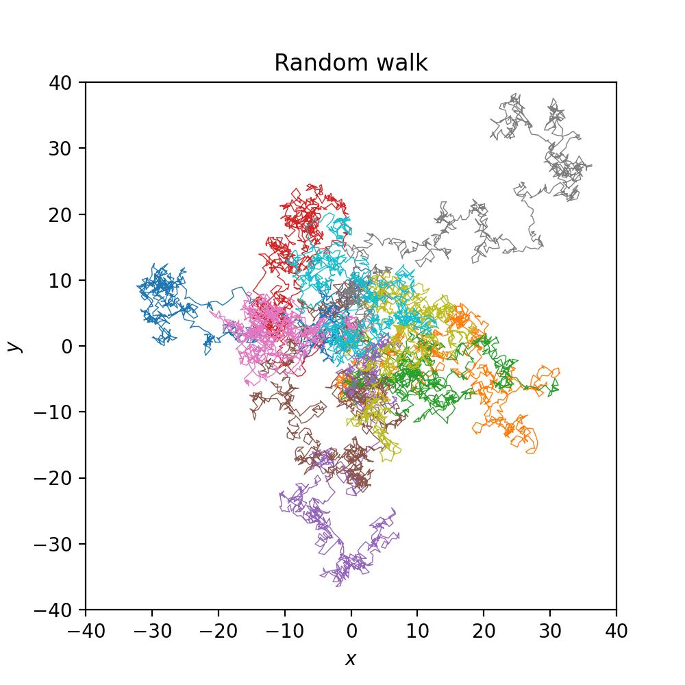
In our random-walk simulation an artificial walker takes sequential steps with the direction of each step independent of the direction of the previous step. For our model, we start at the origin and take steps in the plane of lengths (not coordinates)

The radial distance from the starting point after steps is

If the walk is random, the particle is equally likely to travel in any direction at each step. If we take the average of a large number of such random steps, all the cross terms in will vanish and we will be left with

Implementation: Random Walk

import numpy as np
import matplotlib.pyplot as plt
import random

N = 1000
repeat = 10
x_start, y_start = 0, 0
x, y = [0], [0]

plt.figure(figsize=(5, 5))
plt.xlim(-40, 40)
plt.ylim(-40, 40)
plt.xlabel("$x$")
plt.ylabel("$y$")
plt.title("Random walk")

for i in range(repeat):
    for j in range(N):
        x_start += (random.random() - 0.5) * 2
        y_start += (random.random() - 0.5) * 2
        x.append(x_start)
        y.append(y_start)
    plt.plot(x, y, linewidth=0.5)
    x_start, y_start = 0, 0
    x, y = [0], [0]
    
plt.savefig("walk.jpg", dpi=200)

Spontaneous Decay (Problem)

The probability of decay of any one particle in any time interval is constant, just when it decays is a random event.

Discrete Decay (Model)

Imagine having a sample containing radioactive nuclei at time . Let be the number of particles that decay in some small time interval . We convert the statement “the probability of any one particle decaying per unit time is a constant” into the equation


where the constant is called the decay rate and the minus sign indicates a decreasing number. This equation is a finite-difference equation relating the experimentally quantities , , and

Continuous Decay (Model)

When the number of particles and the observation time interval , our difference equation becomes a differential equation, and we obtain the familiar exponential decay law

We see from its derivation that the exponential decay is a good description of nature for a large number of particles where .

Decay Simulation

import matplotlib.pyplot as plt
import numpy as np

lambda_ = 0.01
particles = 200
end_time = 500
number = particles
res = []
for i in range(end_time):
    decay = np.random.rand(number)
    gone = (decay < lambda_).sum()
    number -= gone
    res.append(number)

plt.figure(figsize=(5, 4))
plt.plot(range(end_time), res, "b-", linewidth=0.8)
plt.xlabel("$t$")
plt.ylabel("Number left")
plt.title("Spontaneous Decay")
plt.yscale("log")
plt.savefig("decay.jpg", dpi=200)